Machine Learning in Finance

Subheading

Certainly! Random forests are a clever method in machine learning where several decision trees team up to make predictions. They’re really interesting because they’re super accurate, can handle both classifying things and predicting values, and they’re great at avoiding mistakes that come from being too focused on the training data. Plus, you don’t have to tweak a lot of settings to make them work well, which makes them really handy and flexible in the world of data science and predictive modeling.

Classification and Random Forests

Classification forecasting with time series refers to the application of classification algorithms to predict categorical outcomes or classes based on historical time series data. In this context, time series data refers to sequential observations collected over time, and classification forecasting aims to categorize future data points or time periods into predefined classes or categories.

In classification forecasting, the goal is to predict a categorical outcome or target variable based on historical time series data. This categorical outcome can take on discrete class labels, such as “up” or “down” for stock price movement, “normal” or “anomalous” for sensor readings, or any other relevant categories.

Random forests are a highly effective type of ensemble learning used for classifying and predicting values. They’re part of decision tree-based algorithms and are famous for their adaptability, stability, and capability to manage intricate data.

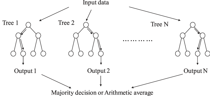
In random forests, several decision trees collaborate to enhance accuracy and reliability in predictions. The concept behind ensemble learning is simple: when you merge outcomes from numerous models, you often get superior performance compared to using just one model.

At the core of a Random forest are decision trees. Decision trees are a type of supervised machine learning model that makes decisions by partitioning the input data into subsets based on specific feature values and creating a tree-like structure of decision nodes. Random forests employ a technique called Bootstrap aggregating, or Bagging for short. Bagging involves creating multiple random subsets (with replacement) of the original dataset.

Each subset is used to train an individual decision tree. This process reduces the variance and helps prevent overfitting because each tree sees a slightly different version of the data. In addition to using bootstrapped samples, Random forests introduce randomness by selecting only a random subset of features at each node of the decision tree. This helps to decorrelate the trees and further increase the model’s robustness.

Once all the individual decision trees are trained, they are combined to make predictions. For classification tasks, each tree “votes” for a class, and the class with the most votes becomes the final prediction.

The following illustration shows how a random tree works.

Creating the Algorithm

The classification task will use a financial time series example, the S&P 500. Here’s the plan of attack:

• Import daily S&P 500 index values in Python.
• Make the data stationary by taking the differences between each closing price and the one preceding it.
• Categorize the data with positive differences being labeled as 1 and negative differences being labeled as -1.
• Create an array that holds the categorical variables with lags that go as far as 50 (this suggests you will have multiple-column arrays).
• Fit the random forest model on the training set.
• Predict on the test set using the fitted model.
• Evaluate the results using accuracy (number of variables that match between the predicted and the real variables from the test set) and Cohen’s Kappa (defined below).

The full code to do this is as follows (keep in mind that you must pip install pandas_datareader from the prompt):import numpy as np
from sklearn.model_selection import train_test_split
from sklearn.ensemble import RandomForestClassifier
from sklearn.metrics import accuracy_score, cohen_kappa_score
import pandas_datareader as pdr
import matplotlib.pyplot as plt

def data_preprocessing(data, num_lags, train_test_split):
# Prepare the data for training
x = []
y = []
for i in range(len(data) – num_lags):
x.append(data[i:i + num_lags])
y.append(data[i+ num_lags])
# Convert the data to numpy arrays
x = np.array(x)
y = np.array(y)
# Split the data into training and testing sets
split_index = int(train_test_split * len(x))
x_train = x[:split_index]
y_train = y[:split_index]
x_test = x[split_index:]
y_test = y[split_index:]

return x_train, y_train, x_test, y_test

start_date = ‘1960-01-01’
end_date = ‘2023-09-01’

# Set the time index if it’s not already set
data = (pdr.get_data_fred(‘SP500’, start = start_date, end = end_date).dropna())

# Perform differencing to make the data stationary
data_diff = data.diff().dropna()

# Categorizing positive returns as 1 and negative returns as -1
data_diff = np.reshape(np.array(data_diff), (-1))
data_diff = np.where(data_diff > 0, 1, -1)

x_train, y_train, x_test, y_test = data_preprocessing(data_diff, 50, 0.80)

# Create and train a Random Forest Classifier
model = RandomForestClassifier(n_estimators = 100, random_state = 0)
model.fit(x_train, y_train)

# Make predictions
y_predicted = model.predict(x_test)

# Evaluate the model
accuracy = accuracy_score(y_test, y_predicted)
kappa = cohen_kappa_score(y_test, y_predicted)
print(f”Accuracy: {accuracy:.2f}”)
print(f”Kappa: {kappa:.2f}”)

The output of the code is as follows:Accuracy: 0.55
Kappa: 0.10

This simple model achieved 55% accuracy on categorical up or down data with a Cohen’s Kappa of 0.10.

Cohen’s Kappa is a measure of agreement that quantifies the degree of agreement between two raters or evaluators beyond what would be expected by random chance. The interpretation can vary, but here are some common guidelines for assessing the level of agreement:

1. Below zero: Indicates less agreement than would be expected by chance. There may be systematic disagreement between the raters.
2. Between zero and 0.20: Indicates slight agreement. The agreement is only slightly better than what would be expected by random chance.
3. Between 0.21 and 0.40: Indicates fair agreement. The agreement is moderate but still may be improved.
4. Between 0.41 and 0.60: Indicates moderate agreement. The agreement is substantial and generally considered acceptable.
5. Between 0.61 and 0.80: Indicates substantial agreement. The agreement is strong, and there is a high level of consistency between the raters.
6. Between 0.81 and 1.00: Indicates almost perfect agreement. The agreement is very high, and there is near-perfect consistency between the raters.

The appropriate level of agreement may be influenced by factors such as the consequences of misclassification and the difficulty of the classification task.